Linear regression part two - finding the covariance of the quadratic loss minimizing line under homoskedasticity.

Last time, I began with a graph.

Namely, this one:

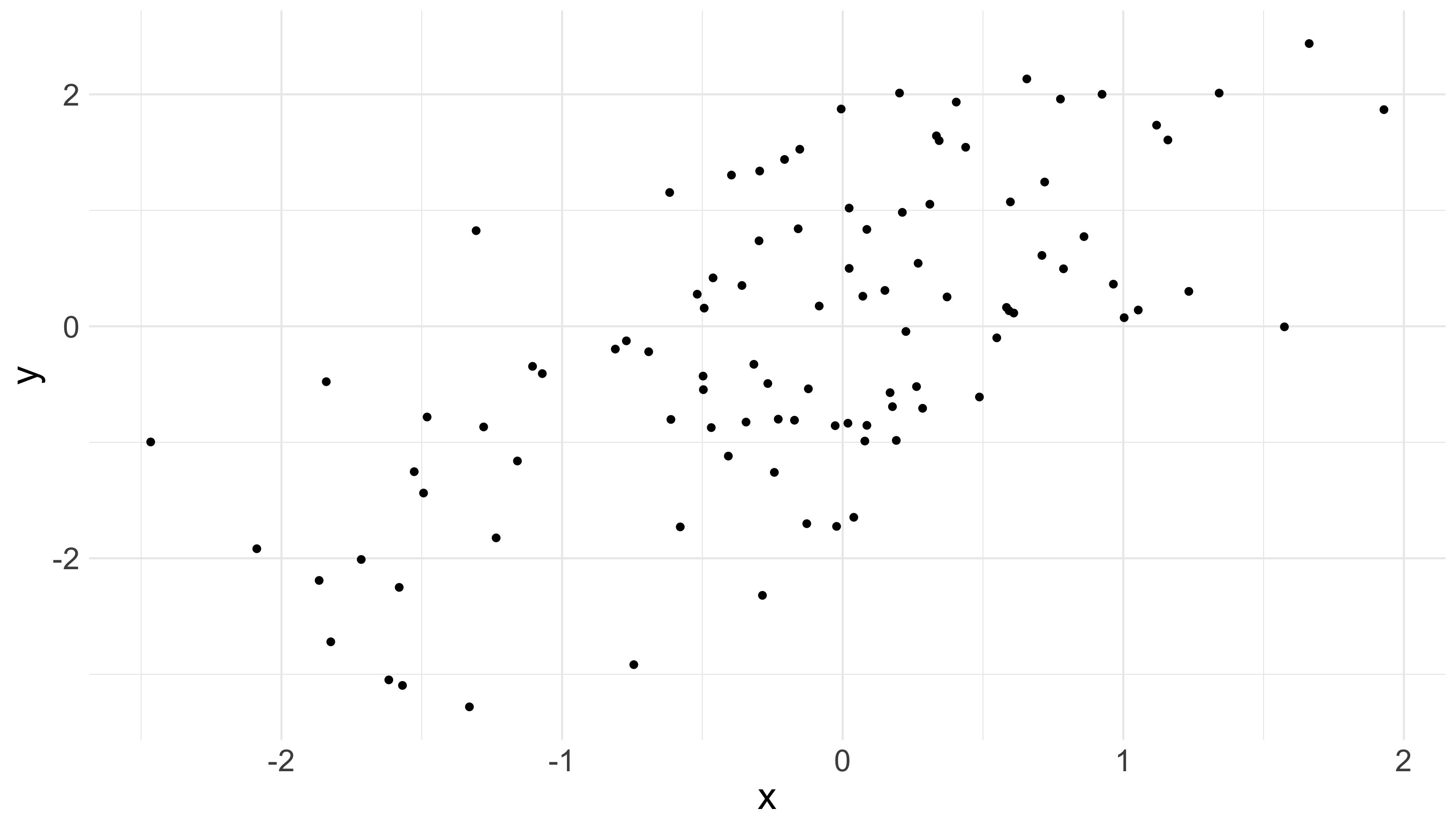
And we regarded the points on that graph as fixed, and found the linear function of $x$ which minimized quadratic loss for those points. Recall we assumed nothing stochastic; we were just minimizing a loss function taken over fixed data. And recall also that if we let

$$\begin{align*} Y = \begin{bmatrix} y_1 \\ y_2 \\ \vdots \\ y_n \end{bmatrix}, \quad \text{and} \quad X = \begin{bmatrix} 1 & x_1 \\ 1 & x_2 \\ \vdots & \vdots \\ 1 & x_n \end{bmatrix} \end{align*}$$

then we found that the vector

$$\hat{\beta} = (X'X)^{-1}X'Y$$

supplies the line which minimizes quadratic loss for our data. Its first element is the intercept, and its second is the slope.

But typically, we do not think of our data as fixed. Instead, we see each data point as a realization from a chance process – a realization from a joint probability distribution, $P(x, y)$, governing $x$ and $y$. (We might, for example, think of $x$ as weight, and $y$ as height, and then imagine selecting someone at random. $P(x,y)$ would then describe the probability of selecting a person of weight $x$ and height $y$.)

And if we do see our data as realizations from a chance process, then we might wonder: if we had seen alternative realizations from $P(x,y)$, how would we expect our quadratic-loss-minimizing line to have differed? The below picture, for example, shows two 100 data point samples from the same underlying distribution on $x$ and $y$, along with the quadratic-loss-minimizing lines for each:

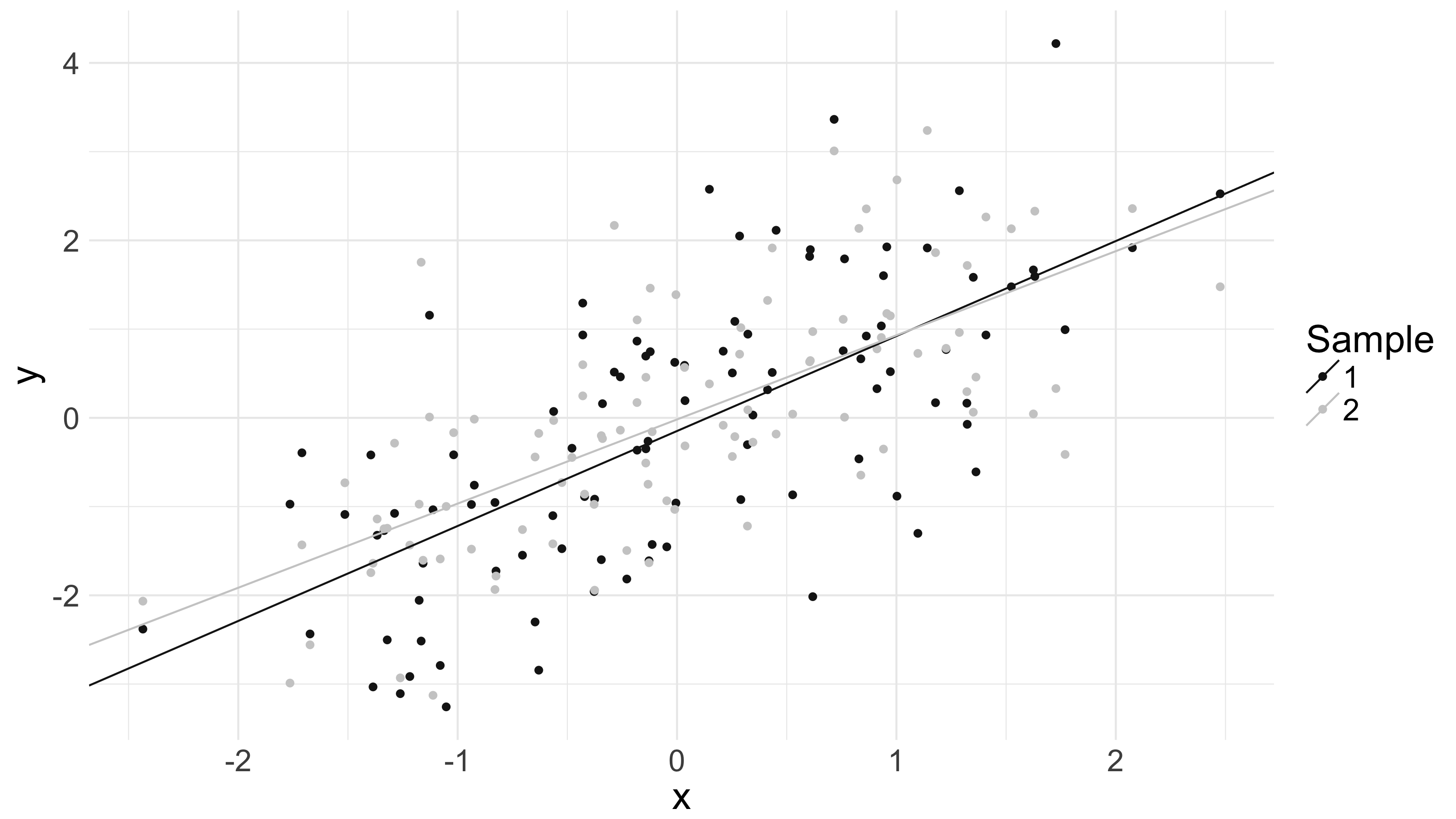
Appreciate how they shift and vary.

Now, we might also wonder: if we regard our $x$-values as fixed, how would we expect our quadratic-loss-minimizing line to have varied? That is, how would we expect them to vary given alternative realizations from $P(y \vert x)$?

The below picture shows 20 100-data point samples from the same distribution $P(y \vert x)$, along with quadratic-loss-minimizing lines for each:

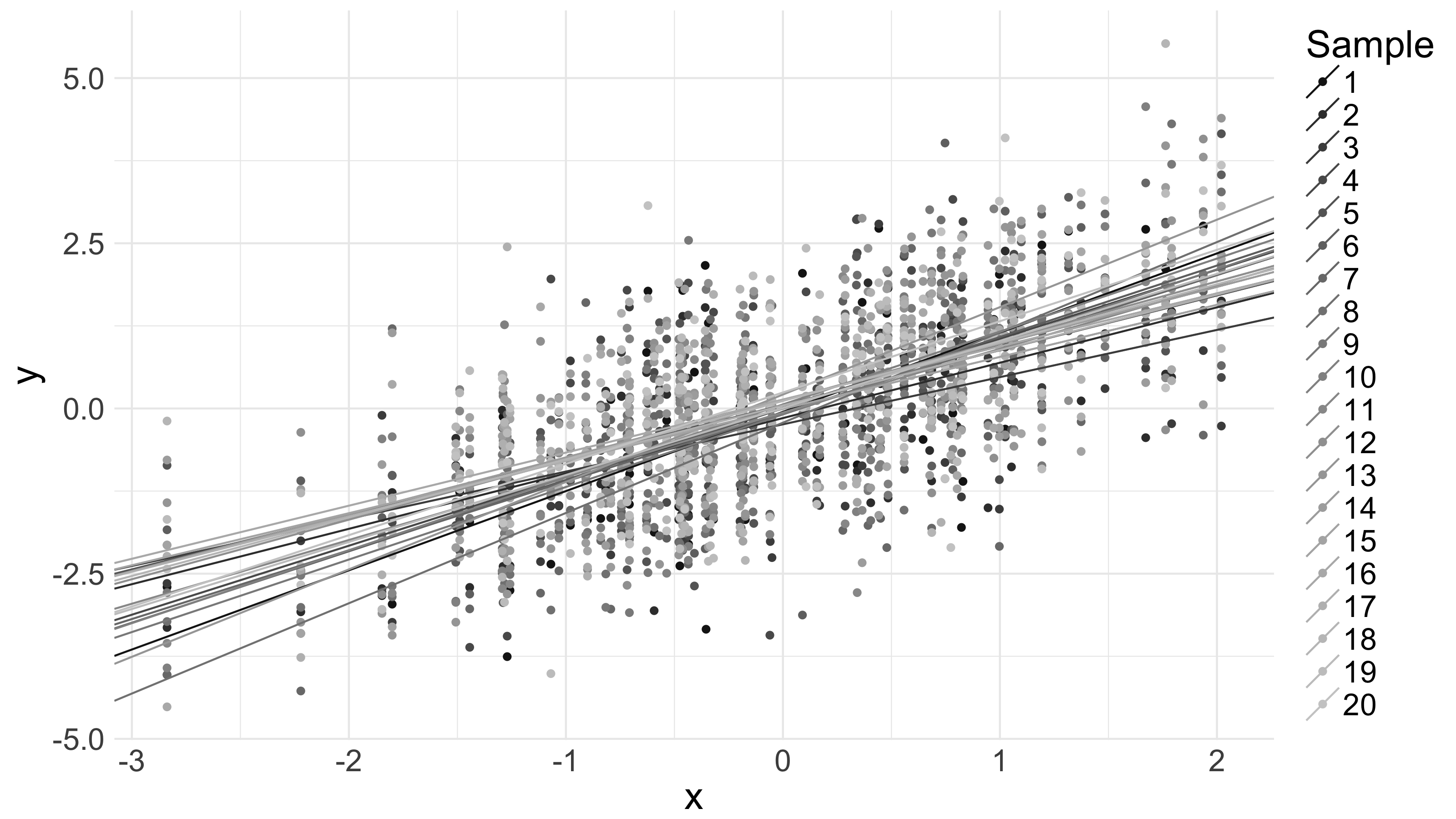
Appreciate, again, how they shift and vary. Notice also the vertical striations in the data on the graph. These are a result of the fact that the vector of $x$-values is fixed, and I’ve sampled $y$ from around those fixed $x$-values.

The difference between the first question – ‘how would I expect the lines to vary if I saw alternative realizations from $P(x,y)$?’ – and the second question – ‘how would I expect the lines to vary if I saw alternative realizations from $P(y \vert x)$?’ – is subtle. The first asks – across samples from $P(x,y)$, how do quadratic-loss-minimizers tend to vary. The second asks – across all samples from $P(x,y)$ where the vector of $x$ values is equal to the vector of $x$-values I happened to witness – how do quadratic-loss-minimizers tend to vary? Here, we’ll focus on this latter question, mostly because it’s easier to answer, but also because it’s more relevant, given we saw the data we did.

Now, without knowing the distribution $P(y \vert x)$ it’s hard to say much about the variation we should expect in our quadratic-loss-minimizing lines. But we can make the problem tractable by imposing some additional constraints.

For example, assume that, conditional on the vector of $x$-values, each response $y_i$ is independent of every other response $y_j$. Assume also that – again conditional on the vector of $x$-values – the variance of the responses $y_i$ is constant, and denote that constant variance by ‘$\sigma^2$’. In other words, assume that for the vector $Y$ of $y$ values, $cov(Y \vert X) = \sigma^2 I$.

Given that assumption, we can compute the covariance matrix of $\hat{\beta}$ as follows:

$$\begin{align*} cov (\hat{\beta} | X) &= E[(\hat{\beta} - E(\hat{\beta}))(\hat{\beta} - E(\hat{\beta}))' | X] \\ &= E\big[\big(X'X)^{-1}X'Y - E((X'X)^{-1}X'Y)\big) \big((X'X)^{-1}X'Y - E((X'X)^{-1}X'Y)\big)' | X] \\ &= E[(X'X)^{-1}X'YY'X(X'X)^{-1} - \\ & \quad \qquad (X'X)^{-1}X'E(Y)Y'X(X'X)^{-1} - \\ & \quad \qquad (X'X)^{-1}X'YE(Y)'X(X'X)^{-1} + \\ & \quad \qquad (X'X)^{-1}X'E(Y)E(Y)'X(X'X)^{-1} | X] \\ &= (X'X)^{-1}X'E\big[YY' - E(Y)Y' - Y'E(Y)' + E(Y)E(Y)' | X \big]X(X'X)^{-1} \\ &= (X'X)^{-1}X'\underbrace{E\big[(Y - E(Y))(Y - E(Y))' | X]}_{cov (Y | X)}X(X'X)^{-1} \\ &= (X'X)^{-1}X'\sigma^2IX(X'X)^{-1} \\ &= \sigma^2 (X'X)^{-1}X'X(X'X)^{-1} \\ &= \sigma^2 (X'X)^{-1} \end{align*}$$

I think the generality of this result somewhat surprising, because it only relies on conditional independence and constant variance. Consider the below picture. It shows 20 100-data-point samples from a fixed-conditional-variance distribution, where $E(y \vert x) = x^3$, along with 20 corresponding quadratic-loss-minimizing lines:

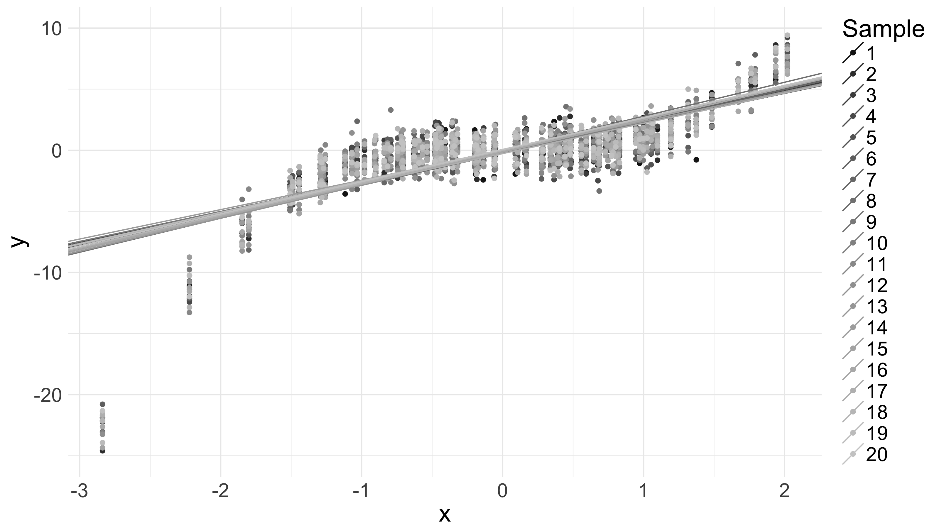
Now, compare that picture to a similar picture below – with the same $x$-values, but where the $y$-values are generated from a distribution with $E(y \vert x) = x$ – i.e., where the conditional mean of $y$ is a linear, instead of a cubic, function of $x$:

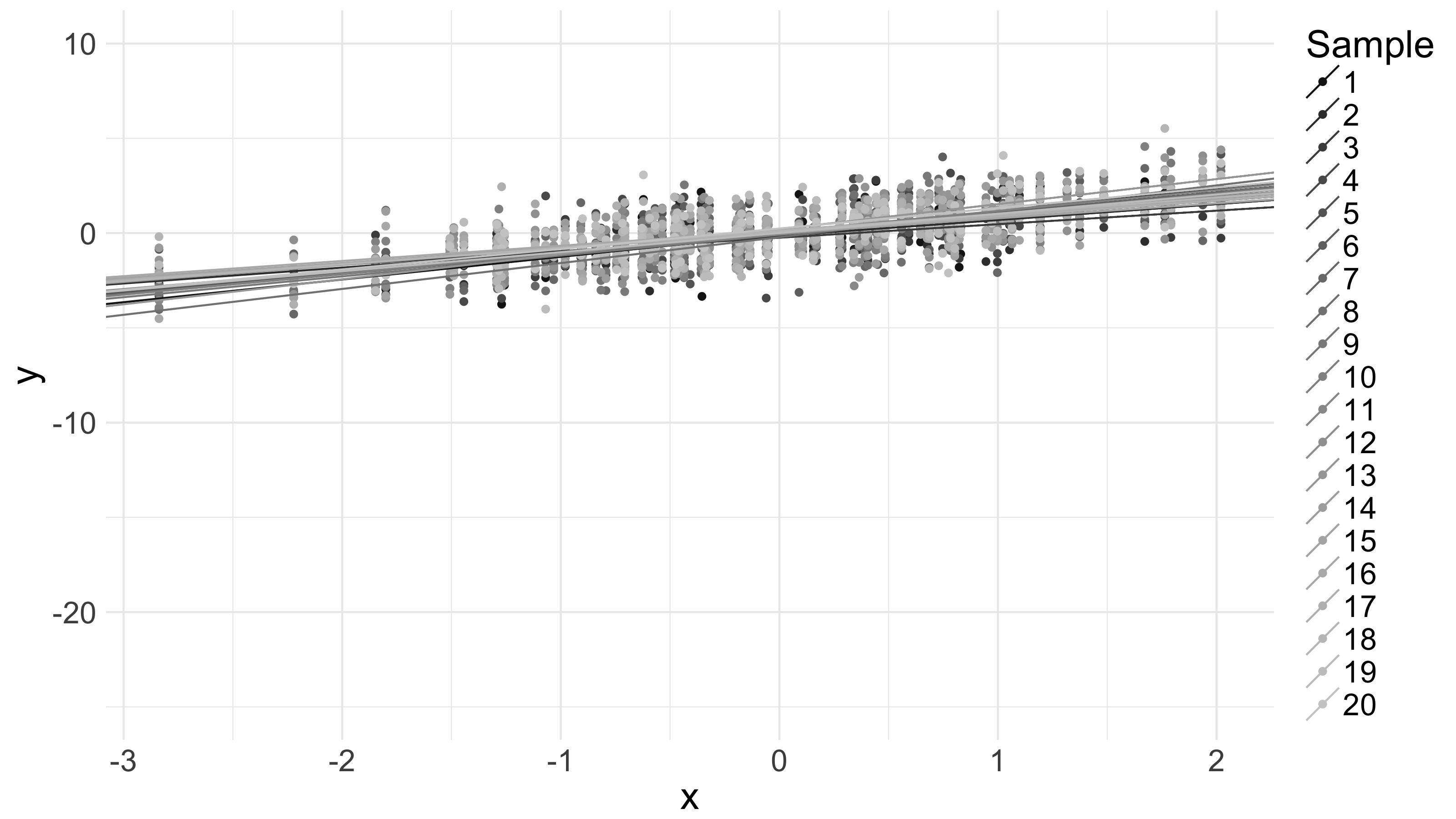
We see generally different slopes across the two plots. That’s not surprising. But consider: both plots are on the same scale, and the variation in the quadratic-loss-minimizing lines is (approximately) the same in both cases. This, despite the fact that the conditional mean of $y$ is a much more complicated function of $x$ in the former case than in the latter.

I think that last is surprising. More precisely, I think it surprising that the covariance matrix of $\hat{\beta}$ – which expresses the amount of variation in our quadratic-loss-minimizing lines – is independent of $E(y \vert x)$ considered as a function of $x$. Under every such function the expected variation in our quadratic-loss-minimizing lines is the same.

That’s enough for now; something that is also surprising is that there is still more to say about drawing straight lines through a crop of data points. So, still more to come on this.

---

Code below: generate 20 100-data-point samples from the same conditional distribution, and plot quadratic-loss-minimizers for each.

require(ggplot2)

## Init structures to store samples
df <- NULL
beta_hat <- NULL

## Generate some x-values. X[,2] ~ N(0, 1)
X <- matrix(c(rep(1, 100), rnorm(100)), ncol = 2)

## Over 20 iterations, generate 100 y-values, Y ~ N(X[,2], 1), 
## and compute quadratic-loss-minimizers
for (i in seq(1:20)){
  Y <- rnorm(100, mean = X[,2])
  df <- rbind.data.frame(df, cbind.data.frame(x = X[,2], 
  					      y = Y, 
  					      iter = i))
  
## Find (X'X)^(-1)X'Y.
  bh <- solve(t(X) %*% X) %*% t(X) %*% Y
  beta_hat <- rbind.data.frame(beta_hat, 
                               cbind.data.frame(intercept = bh[1], 
                               slope = bh[2], 
                               iter = i))
}

## Plot the samples along with their quadratic-loss-minimizers.
ggplot(df, aes(x = x, y = y, color = as.factor(iter))) + 
  geom_point() + 
  theme_minimal() +
  scale_color_grey(start = 0.1, name = 'Sample') + 
  theme(text = element_text(size = 20)) +
  geom_abline(data = beta_hat,
              aes(intercept = intercept, slope = slope, color = as.factor(iter)))